Gaussian Data

In this notebook, we want to demonstrate how to use Entropy (H) and Mutual Information (MI), and showcase the different approaches on gaussian random data.

import infomeasure as im
import numpy as np
import matplotlib.pyplot as plt
rng = np.random.default_rng(29615)

2026-04-01 12:37:26,326 |     INFO | font_manager.py:1107 | Failed to extract font properties from /usr/share/fonts/truetype/noto/NotoColorEmoji.ttf: Can not load face (unknown file format; error code 0x2)

2026-04-01 12:37:26,508 |     INFO | font_manager.py:1639 | generated new fontManager

Entropy

Generate normal distributed random variables with varying standard deviation \(\sigma\).

n = 500
stds = np.linspace(0.1, 10, 20)  # standard deviations to test
# data is an array of shape (len(stds), n)
data_h = rng.normal(0, stds[:, None], (len(stds), n))

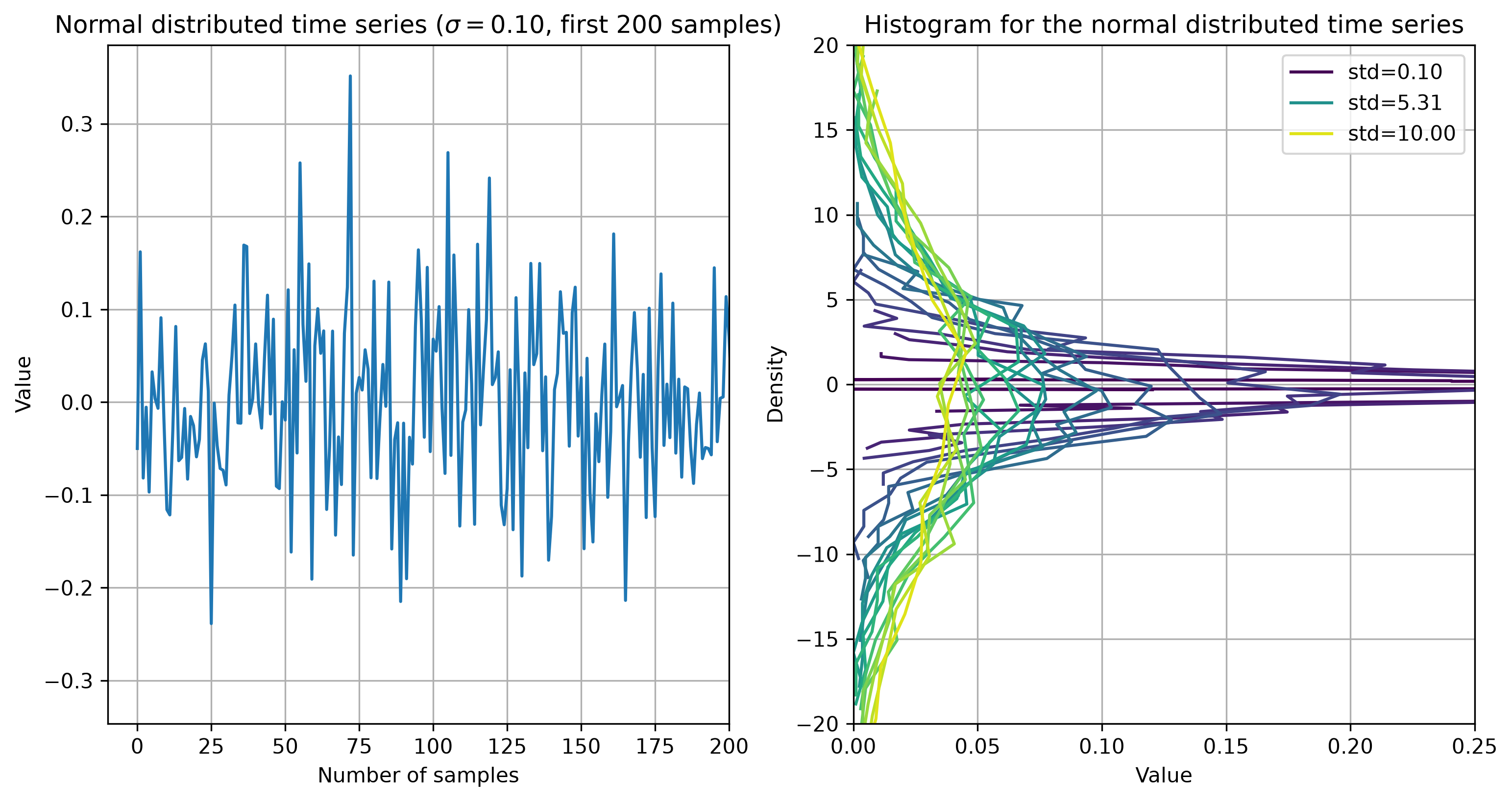
Let’s look at the first time series and plot the first 200 samples. Also, compare the histograms of the time series for different \(\sigma\) values.

Show code cell source

Hide code cell source

fig, axes = plt.subplots(1, 2, figsize=(12, 6), dpi=300)

m = 200
axes[0].plot(data_h[0])
axes[0].grid()
axes[0].set_xlabel('Number of samples')
axes[0].set_xlim(-10, m)
axes[0].set_ylabel('Value')
axes[0].set_title(
    fr'Normal distributed time series ($\sigma={stds[0]:.2f}$, first {m} samples)')

cmap = plt.get_cmap('viridis')
for i in range(len(stds)):
    hist, bins = np.histogram(data_h[i], bins=20, density=True)
    axes[1].plot(hist, bins[:-1], color=cmap(i / len(stds)), label=(f'std={stds[i]:.2f}' if i in [0, len(stds)//2, len(stds)-1] else None))
axes[1].set_ylim(-20, 20)
axes[1].set_xlim(0, 0.25)
axes[1].set_xlabel('Value')
axes[1].set_ylabel('Density')
axes[1].set_title(
    fr'Histogram for the normal distributed time series')
axes[1].legend()
axes[1].grid()

plt.show()

To compare with an expected value, we can calculate the analytical entropy for each \(\sigma\) value:

\[ H(X) = \frac{1}{2} \log(2\pi e \sigma^2) \]

def analytical_entropy(sigma, base=im.Config.get('base')):
    """Analytical entropy of a normal distributed random variable
    with standard deviation sigma."""
    h = 0.5 * np.log(2 * np.pi * np.e * sigma ** 2)
    if base == 'e':
        return h
    return h / np.log(base)

This is the value we should expect when calculating the global value for the different approaches. To compute the numerical entropy for all approaches, loop over each \(\sigma\) value and approach. For the discrete approach, the values need to be discretized to integers.

approaches = {
    'discrete': {},
    'kernel': {'bandwidth': 0.5, 'kernel': 'box'},
    'metric': {'k': 4, 'minkowski_p': 2},
    'renyi': {'alpha': 1},  # alpha=1 is the Shannon entropy
    'ordinal': {'embedding_dim': 2},
    'tsallis': {'k': 4, 'q': 1},  # q=1 is the Shannon entropy
    'miller_madow': {},
    'bayes': {'alpha': 0.5},
    'shrink': {},
    'grassberger': {},
    'chao_wang_jost': {},
    'ansb': {'undersampled': np.inf},
    'nsb': {},
    'zhang': {},
    'bonachela': {},
}
entropies = np.zeros((len(approaches), len(stds)))
for i, std in enumerate(stds):
    for j, name, kwargs in zip(range(len(approaches)), approaches.keys(),
                               approaches.values()):
        if name in ['kernel', 'metric', 'renyi', 'ordinal', 'tsallis']:
            entropies[j, i] = im.entropy(data_h[i], approach=name, **kwargs)
        else:  # discrete / continuous
            if name in ['nsb', 'ansb']:
                kwargs['K'] = max(1,int(len(data_h[i].astype(int))/100))
            entropies[j, i] = im.entropy(data_h[i].astype(int), approach=name, **kwargs)

/home/docs/checkouts/readthedocs.org/user_builds/infomeasure/checkouts/latest/infomeasure/estimators/entropy/nsb.py:116: RuntimeWarning: overflow encountered in exp
  exp(-self._neg_log_rho(beta, K, N, counts) + l0)
/home/docs/checkouts/readthedocs.org/user_builds/infomeasure/checkouts/latest/infomeasure/estimators/entropy/nsb.py:116: RuntimeWarning: invalid value encountered in scalar multiply
  exp(-self._neg_log_rho(beta, K, N, counts) + l0)
/home/docs/checkouts/readthedocs.org/user_builds/infomeasure/checkouts/latest/infomeasure/estimators/entropy/nsb.py:114: IntegrationWarning: The occurrence of roundoff error is detected, which prevents 
  the requested tolerance from being achieved.  The error may be 
  underestimated.
  numerator, _ = quad(
/home/docs/checkouts/readthedocs.org/user_builds/infomeasure/checkouts/latest/infomeasure/estimators/entropy/nsb.py:130: RuntimeWarning: overflow encountered in exp
  exp(-self._neg_log_rho(beta, K, N, counts) + l0)

infomeasure enables us to use the im.entropy() function, passing the approach-name and additional keyword arguments for the corresponding approach. Like this, the single call im.entropy(data_h[i], approach='discrete') already computes the entropy of a discrete distribution. Let’s plot the entropy for each approach and \(\sigma\) value, while comparing it with the expected analytical entropy:

Show code cell source

Hide code cell source

# Compute analytical values (higher precision)
analytical_stds = np.linspace(min(stds) / 10, max(stds), 100)
analytical_entropies = np.array([analytical_entropy(std) for std in analytical_stds])
analytical_entropies_stds = np.array([analytical_entropy(std) for std in stds])

# Plot results
fig = plt.figure(figsize=(8, 5), dpi=300)
colors = plt.cm.tab20(np.linspace(0, 1, len(approaches)))
for i, name in enumerate(approaches.keys()):
    plt.plot(stds, entropies[i], label=name, marker='o', linewidth=6 - i / 3., color=colors[i])

# Analytical values
plt.plot(analytical_stds, analytical_entropies, label='Analytical', linewidth=1.8,
         color='black')

plt.xlabel(r'Standard deviation $\sigma$')
plt.ylabel('Entropy')
plt.ylim(-1, 7)
plt.title('Entropy estimation of Gaussian data')
plt.legend(bbox_to_anchor=(1.05, 1), loc='upper left', ncol=1)
plt.grid()
plt.show()

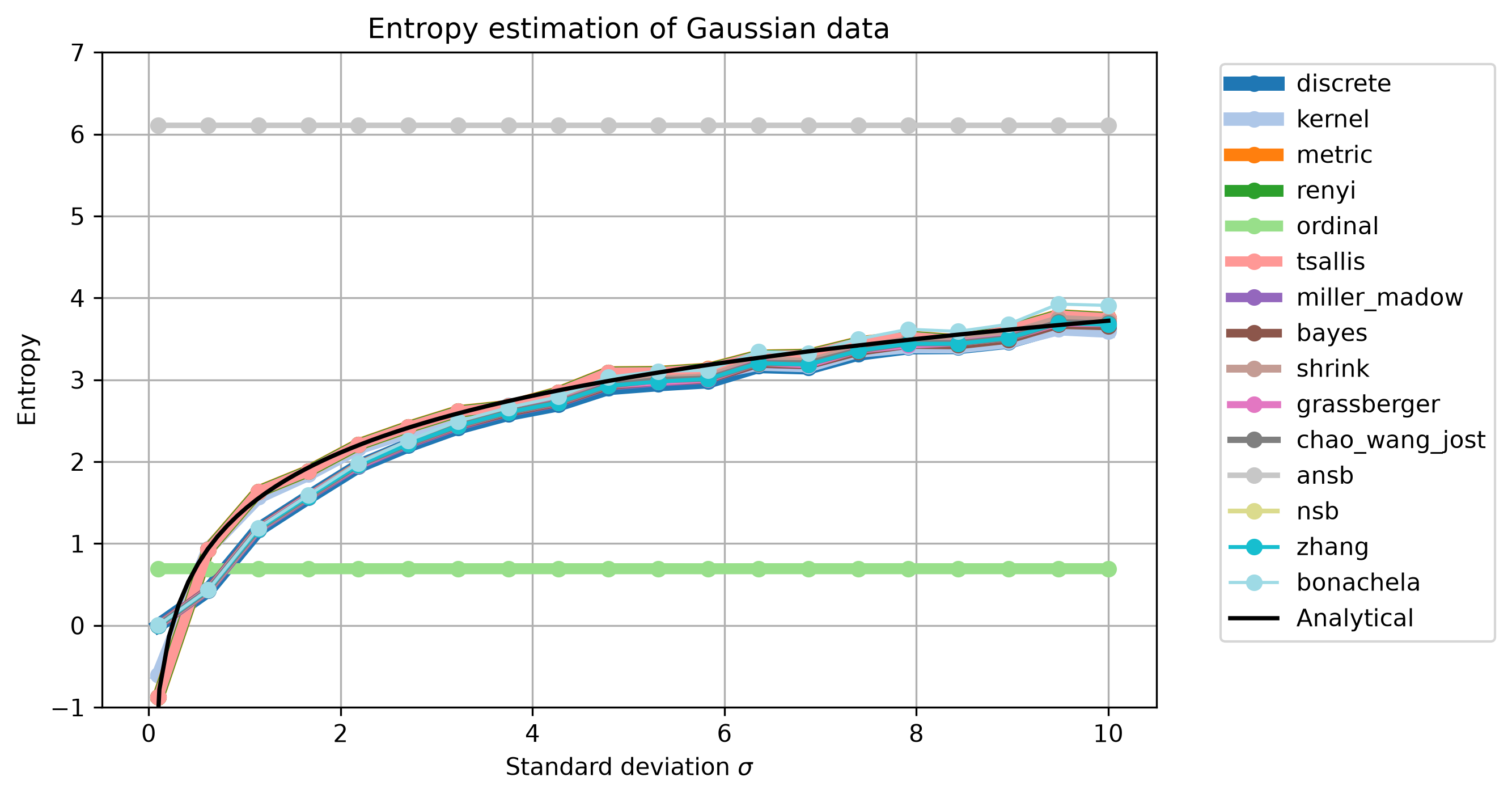
All methods match the analytical values very closely, except the ordinal and ansb one. For the discrete estimators, the discretization leads to a deviation at lower \(\sigma\). For \(\sigma = 0.1\) all values get converted to 0, producing entropy of 0. The ordinal method returns constant values. This is to be expected because the symbolization is independent of \(\sigma\), as the distributions of ordinal patterns are invariant under scaling. ansb is not resembling the analytical value as the data is not undersampled enough.

Show code cell source

Hide code cell source

# Plot the percentage error of the estimated entropy compared to the analytical value
fig = plt.figure(figsize=(8, 3), dpi=300)
symbols = ['o', 's', 'd', '^', 'v', 'x', 'h', 'p', '*', '+', '1', '2', '3', '4']
for i, name in enumerate(approaches.keys()):
    plt.plot(stds,
             100 * (entropies[
                        i] - analytical_entropies_stds) / analytical_entropies_stds,
             label=name, marker=symbols[i % len(symbols)], markersize=10,
             linewidth=2, linestyle='--', color=colors[i])
# horizontal line at 0
plt.axhline(0, color='black', linewidth=2, zorder=-1)
plt.xlabel(r'Standard deviation $\sigma$')
plt.ylabel(r'Percentage error (%)')
plt.ylim(-20, 15)
plt.legend(bbox_to_anchor=(0.5, 1.15), loc='center', ncol=4)
plt.grid()
plt.show()

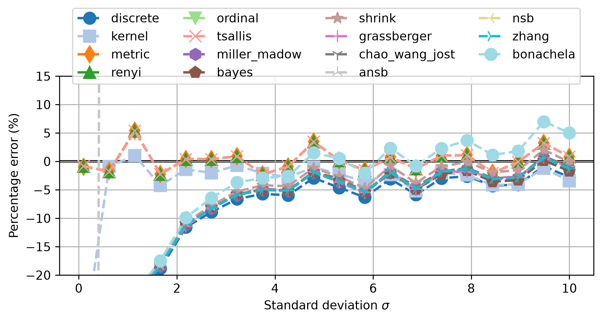
ordinal is off the charts, mostly around \(-75\%\).

Mutual Information

For Mutual Information (MI), we demonstrate the measures with multivariate Gaussian data, varyig the correlation coefficient \(\rho\). Analytically, the mutual information between two gaussian random variables \(X\) and \(Y\) with zero mean and unit variance is given by

\[ I(X; Y) = -\frac{1}{2} \log(1 - \rho^2). \]

# Analytical formula for the mutual information of two Gaussian random variables
def mutual_information_gauss(X, Y):
    """Compute the mutual information between two Gaussian random variables.

    Notes
    -----
    ``r`` is the correlation coefficient between X and Y.
    ``I_Gauss`` is the mutual information between X and Y.
    """
    r = np.corrcoef(X, Y)[0, 1]
    I_Gauss = -0.5 * np.log(1 - r ** 2)
    return I_Gauss

Show code cell source

Hide code cell source

def generate_data(N, r):
    cov_matrix = [[10, r], [r, 10]]
    data = np.random.multivariate_normal([0, 0], cov_matrix, N)
    X = data[:, 0]
    Y = data[:, 1]
    return X, Y

# Values of r
r_values = np.linspace(1, 9, 9)
# Number of data points
N = 1000
# Generate data for each r value. shape (len(r_values), 2, N)
data_mi = np.array([generate_data(N, r) for r in r_values])
data_mi_discrete = data_mi.astype(int)

Show code cell source

Hide code cell source

# Visualize data - plot on top of each-other, low to higher r values
from matplotlib import colormaps
plt.figure(figsize=(8, 4), dpi=300)
ax = plt.gca()
cmap = colormaps.get_cmap('viridis')
norm = plt.Normalize(vmin=min(r_values/10), vmax=max(r_values/10))
for i in range(len(r_values)):
    plt.scatter(data_mi[i][0], data_mi[i][1], color=cmap(norm(r_values[i]/10)), marker='.')
# Colorbar
sm = plt.cm.ScalarMappable(cmap=cmap, norm=norm)
sm.set_array([])
cbar=plt.colorbar(sm, ticks=r_values/10, ax=ax)
cbar.set_label(r'Correlation Coefficient $\rho$')
plt.title(r'Joint Distribution $(X, Y)$ for varying $\rho$')
plt.xlabel('X')
plt.ylabel('Y')
plt.grid()
plt.show()

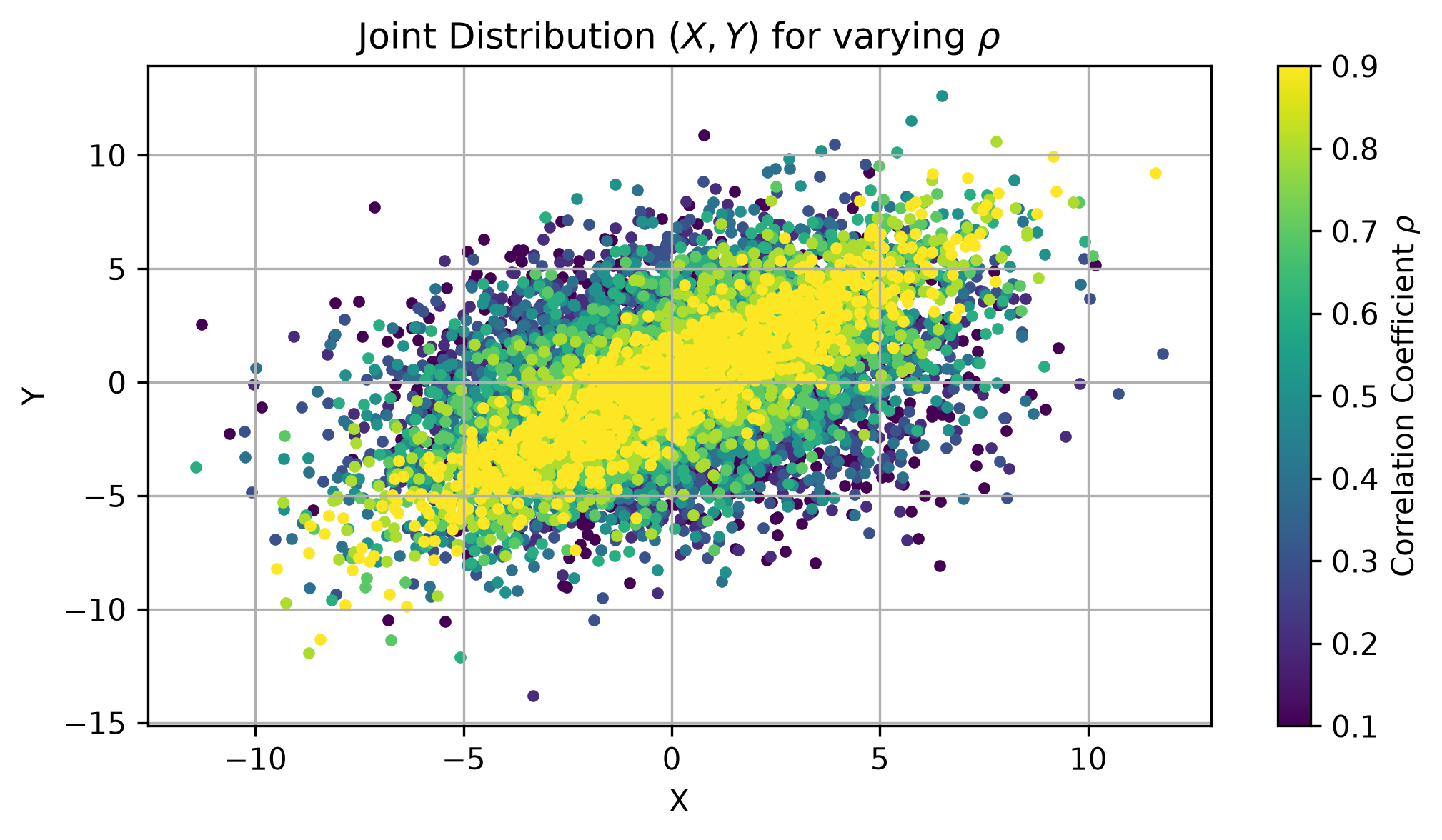
For the lower correlated data points, the scatter plot becomes more scattered. For higher correlated data points, the scatter plot becomes more aligned. Again, prompt the im.mutual_information() function for each approach.

# Compute mutual information for each r value
approaches_mi = {
    # 'ansb': {},
    'bayes': {'alpha': 1.0},
    'bonachela': {},
    'chao_shen': {},
    'chao_wang_jost': {},
    'discrete': {},
    'grassberger': {},
    'kernel': {'bandwidth': 0.5, 'kernel': 'gaussian'},
    'miller_madow': {},
    'nsb': {},
    'metric': {'k': 4},
    'renyi': {'alpha': 0.9},  # alpha=1 is the Shannon entropy
    'shrink': {},
    'ordinal': {'embedding_dim': 3},
    'tsallis': {'k': 4, 'q': 1.05},
    'zhang': {},
}
mi_values = {approach: np.zeros((len(r_values))) for approach in approaches_mi.keys()}
for i, r in enumerate(r_values):
    for name, kwargs in approaches_mi.items():
        if name in ['kernel', 'metric', 'renyi', 'ordinal', 'tsallis']:
            mi_values[name][i] = im.mutual_information(
                data_mi[i][0], data_mi[i][1], approach=name, **kwargs
            )
        else:
            mi_values[name][i] = im.mutual_information(
                data_mi_discrete[i][0], data_mi_discrete[i][1], approach=name, **kwargs
            )

The call of im.mutual_information(data_mi[i][0], data_mi[i][1], approach=name, **kwargs) performs the computation of mutual information between the two variables data_mi[i][0] and data_mi[i][1] using the specified approach with the settings given in kwargs.

Show code cell source

Hide code cell source

# Plot results
fig = plt.figure(figsize=(8, 5), dpi=300)
for i, name in enumerate(approaches_mi.keys()):
    plt.plot(r_values, mi_values[name], label=name, marker='o', linewidth=3, color=colors[i])

# Analytical values
mi_gauss_values = [mutual_information_gauss(data_mi[i][0], data_mi[i][1]) for i in
                   range(len(r_values))]
plt.plot(r_values, mi_gauss_values, label='Analytical', linewidth=1.8, color='black')

plt.xlabel(r'Correlation coefficient ($\rho$)')
plt.ylabel('Mutual Information')
plt.title('Mutual Information vs Correlation Coefficient')
plt.legend()
plt.grid()
plt.show()

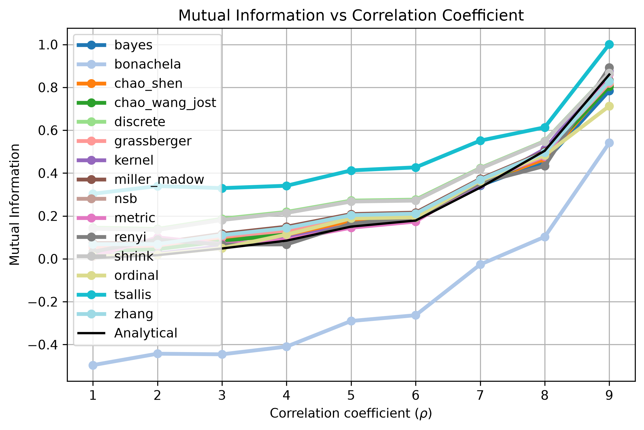
All approaches resemble the expected behaviour of mutual information for Gaussian data. Again, the discrete approaches show offsets, due to discretization errors or dependent whether the data fits the correction term requirements. Tsallis MI is offset as well, because \(q=1.05\) has been used. For \(q=1\), Tsallis MI is identical to Shannon MI. This confirms that the implemented methods correctly estimate the mutual information for Gaussian data.

Conclusion

In this notebook, we have explored various approaches estimating Entropy and Mutual Information for Gaussian data using infomeasure. We also visualised the results and compared them to the analytical expectations. Using this package enables to seamlessly switch estimation approaches and easily find the must suited method for a given dataset and available compute. We focused on the global values of the measures, but not considered the Local Entropy or Local Mutual Information, neither Transfer Entropy (TE). For a transfer entropy demonstration, find the reproduction of the Schreiber’s TE Article [Sch00] on the next page.